

Part of bringing Gzweb to mobiles is improving performance, since mobile devices are typically less powerful than computers. We chose to improve performance by using lower quality 3D models on mobiles.
3D models
 Everyone has an idea of what a 3D model is. We’ve seen them everywhere, from video-games to movies. But what does a 3D model consist of?
- Geometry: a 3D mesh, which in its simplest form consists of coordinates of 3D points (vertices) and information about how they are connected to each other, forming edges and faces.
- Material: how does this model interact with light? Is it shiny, rough?
- Texture: in case the model is not of one single color, an image can be used as its texture.
![]()
The 3D model format used in Gzweb is called COLLADA, which has the extension .dae. COLLADA files may contain not only the 3 components above, but more information about a scene as well, with several models, adding lights, animations and so on. On Gzweb we are mostly interested on a single 3D model contained within a COLLADA file though, since the scene description is made in SDF (Simulation Description Format), which is more suitable for robotics.

There are several open source implementations of mesh simplification out there. We chose to use the GTS library because Gazebo already has a dependency on it. So it should be as simple as adapting their coarsen example to our needs and voilà. Yeah, that’s what I thought a month ago… “Simple”.
Converting, importing, exporting…
GTS simplifies meshes described in its own format. So we must convert COLLADA meshes into GTS surfaces, simplify them, then convert the result back to COLLADA.
COLLADA -> GTS -> simplification -> GTS -> COLLADA
Converting meshes into different formats, wow, that sounds hard! People download whole programs for that, don’t they?
Ok, let’s take advantage of the fact that Gazebo already uses GTS and COLLADA and does some conversion among them. So we add some steps:
COLLADA -> Gazebo -> GTS -> simplification -> GTS -> Gazebo -> COLLADA
That saves us a lot of effort!
- COLLADA -> Gazebo is done with this
- Gazebo -> GTS is based on this
- Simplification is adapted from this
The only part which will need to be written from scratch is exporting back into COLLADA, since Gazebo never had a reason to do this before, there’s no exporter implemented yet.
COLLADA exporter
Structure
COLLADA format is based on XML, which helps organize data in a sort of tree structure. Gazebo’s COLLADA loader uses the TinyXML library to parse the input file. So it makes sense to use the same library to export the simplified mesh. Check out the structure of a really simple COLLADA file:
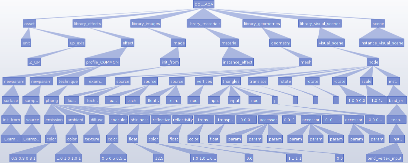
Copy some elements
Luckily, we won’t be exporting a general file here. We’re exporting a simplified version of an existing file. Which means that we can just copy a lot of information from the original file into the new one. Assets, materials, images, effects… All these will be the same in the simplified mesh. What really changes between the original and the simplified version is the geometry.
Geometry element
There are 4 main components of a geometry:
- Vertices: 3D coordinates of each vertex in the mesh (Vx,Vy,Vz)
- Normals: 3D coordinates indicating the direction in which the light is reflected at the vertex (Nx,Ny,Nz)
- Texture map: 2D coordinates indicating a point in the texture file to be linked to a vertex (U,V)
- Faces: this is where all the previous 3 get connected to form faces. We will be working with triangular faces.
Let’s analyze a geometry composed of 2 triangles. The raw texture is shown on the middle.
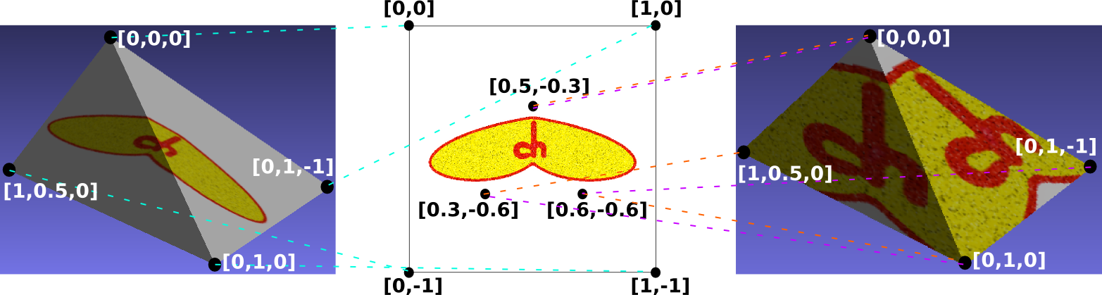
The whole COLLADA file for the figure on the left is here. The texture is here. The following code is where the 4 main geometry components are defined for the figure on the left:
(...)
<float_array count="12" id="Example-Position-array">
0 0   0
1 0.5 0
0 1   0
0 1  -1
</float_array>
(...)
<float_array count="3" id="Example-Normals-array">
0 0 -1
<float_array>
(...)
<float_array count="8" id="Example-UV-array">
0  0
0 -1
1 -1
1  0
</float_array>
(...)
<p>
0 0 0   1 0 1   2 0 2
2 0 2   3 0 3   0 0 0
</p>
(...)
- Vertices: the positions array takes the coordinates for the 4 vertices in the order Vx0 Vy0 Vz0 Vx1 Vy1 Vz1 Vx2 Vy2 Vz2 Vx3 Vy3 Vz3.
- Normals: I chose to use the same normal for all vertices, so there’s only Nx0 Ny0 Nz0.
- Texture map: On this example, I picked the 4 corners of the texture to be U0 V0 U1 V1 U2 V2 U3 V3. For the figure on the right, check the code below.
- Faces: each row corresponds to a triangle. Each group of 3 coordinates refers to a vertex in the triangle, with the indices in order: vertex, normal, texture. So the first triangle has vertex 0 with normal 0 and texture 0, vertex 1 with normal 0 and texture 1 and vertex 2 with normal 0 and texture 2.
The figure on the right uses the exact same positions and normals, but a different texture mapping, shown below. I’ve added this example to show that the same vertex can have different UV for each triangle it is in.
(...)
<float_array count="6" id="Example-UV-array">
0.5 -0.3
0.3 -0.6
0.6 -0.6
</float_array>
(...)
<p>
0 0 0   1 0 1   2 0 2
2 0 2   3 0 3   0 0 0
</p>
(...)
Luckily, we can easily get the simplified mesh’s vertices, normals and face indices. BUT! GTS doesn’t remap the texture to the new geometry! So we gotta do it ourselves…
Texture remapping
Automated texture mapping is no simple task. Several elaborate techniques have been developed, which would take me a while to understand, let alone implement. The key point seems to be trying not to stretch the texture too much. Which is a simple concept, but when you think you’re mapping between a 3D and a 2D space things can get messy.
I thought of doing something simpler, which definitely won’t result in a perfect texture, but should be doable within the time I have. I will just selectively copy the UV coordinates from the original mesh. Let’s pretend this is the original mesh:

But actually, when Gazebo loads it, it makes a mesh composed of unconnected triangles. That is, each vertex belongs to one single face. But how does it look connected then? Well, there are many overlapping vertices… So you think it’s a single vertex but it isn’t:

Why is that important? Well, even though some vertices share the same Vx Vy Vz, and even Nx Ny Nz, they might not share UV. Look at this texture for the PR2:
 Keep that in mind. So… We simplified our mesh, we have a bunch of new vertices… The magenta vertex is one of them.
 We want to decide the UV coordinates for the magenta vertex. What vertex do we copy it from? Well, from the nearest original vertex. (I’m using the nanoflann library to quickly find the nearest vertex). But there are 5 vertices overlapped, the black ones. So which one do we choose? As we saw above, their UV can be completely different…
 We must take into account which triangle we’re working with. The magenta vertex can be part of several triangles, and for each of them we will choose a different UV. At the moment, we’re working with this green one:
 OK, so let’s take the blue triangle pointing at the closest direction to the green one. First we take all the directions:
 Remember, we’re dealing with directions, which are normalized vectors, so when we compare them, we’re looking at them like this. And the green pair is the one which most closely matches the magenta one.
 So this is the closest triangle. The magenta vertex will have the same UV coordinate as the green one.
 So we do this for each of the 3 vertices in each triangle. Note that we’re not picking a UV coordinate for each vertex in the Positions array. The same way as the 2-triangle example all the way on the top of the page, each vertex can be associated to completely different UV coordinates according to the triangle we’re talking about.
Results
Have we got anywhere with all this? Yes, somewhere 🙂 The code where all this is done is here.
Here are some results for the PR2.
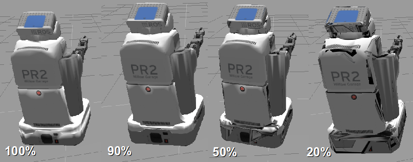
On the left, the mesh with the original number of edges, but with the texture remapped with my crazy method. Yes, remapped, not using the original mapping. And guess what, it has 0% error 😀
The percentage on the other meshes represent how many edges they have with respect to the original. You can see that even cutting down the number of edges by 5 leaves us with a super similar geometry. But with all those overlapping edges that’s not a surprise… They’re the first ones to disappear.
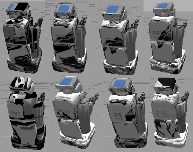
As for the texture mapping, it’s clear that the fewer edges, the more distorted the texture gets. There’s probably a simple way to improve that… Maybe interpolating the UV instead of copying the exact value.
I couldn’t thank my mentor Ian Chen enough. When I started this internship I didn’t understand a single concept described on this page. He has helped me all along the way and been super patient.
To do
Unfortunately, texture mapping is not the only thing to be improved. There are still several problems with the COLLADA exporter. The simplification of some meshes results in errors… For others, even though the simplification goes through, the resulting files are broken. And for several meshes, including the PR2 above, even though they are loaded correctly into Gzweb, their textures don’t show on Meshlab or Sketchup. One thing I’ve learned along the way is that even “standards”, such as COLLADA, are not really seen the same way by everyone.
Bloopers
I know the texture remapping doesn’t look very nice, but hey, it could be worse! I’ve failed a lot before getting here hehehe
